[2] From Maximum Likelihood Estimation (MLE) to Evidence Lower Bound (ELBO): Why Exact Posteriors Are Intractable

Generative Models series: 2. Originally published on Medium.

Post 1 established that training a generative model is equivalent to minimizing KL(P_data ‖ Q_θ). That requires evaluating log Q_θ(x), the likelihood of observed data under the model. For simple models this is tractable, for models with latent variables it isn't.

p(x,z) vs q(z|x)

Source: yunfanj.com

Maximum Likelihood Estimation

Given observed data x and a parameterized model, MLE finds the parameters θ that make the data most probable:

θ = argmax_θ Σ log P(x; θ)

The log converts a product of probabilities into a sum, which is numerically stable and differentiable. For models with a closed-form likelihood (a Gaussian, a categorical distribution) this is straightforward: compute the gradient, update θ, repeat.

MAP estimation extends MLE by placing a prior P(θ) on the parameters. The objective becomes log P(x; θ) + log P(θ), which pulls θ toward a preferred region when data is scarce. Mechanically it is the same optimization, prior adds an extra term to the gradient.

Latent Variable Models

Directly modeling complex distributions like P(image) is hard. A face image has thousands of pixels with intricate statistical dependencies and fitting a single distribution over all of them is computationally heavy and structurally uninformative.

Latent variable models handle this by introducing an unobserved variable z. The generative process is: sample a latent code z from a prior P(z), then sample the observation x from a conditional P(x|z). The marginal probability of x is:

P(x) = ∫ P(x|z) P(z) dz

The latent z captures high-level structure (identity, pose, style) while P(x|z) handles the rendering. This decomposition is useful, but it makes evaluating P(x) intractable.

The Posterior Problem

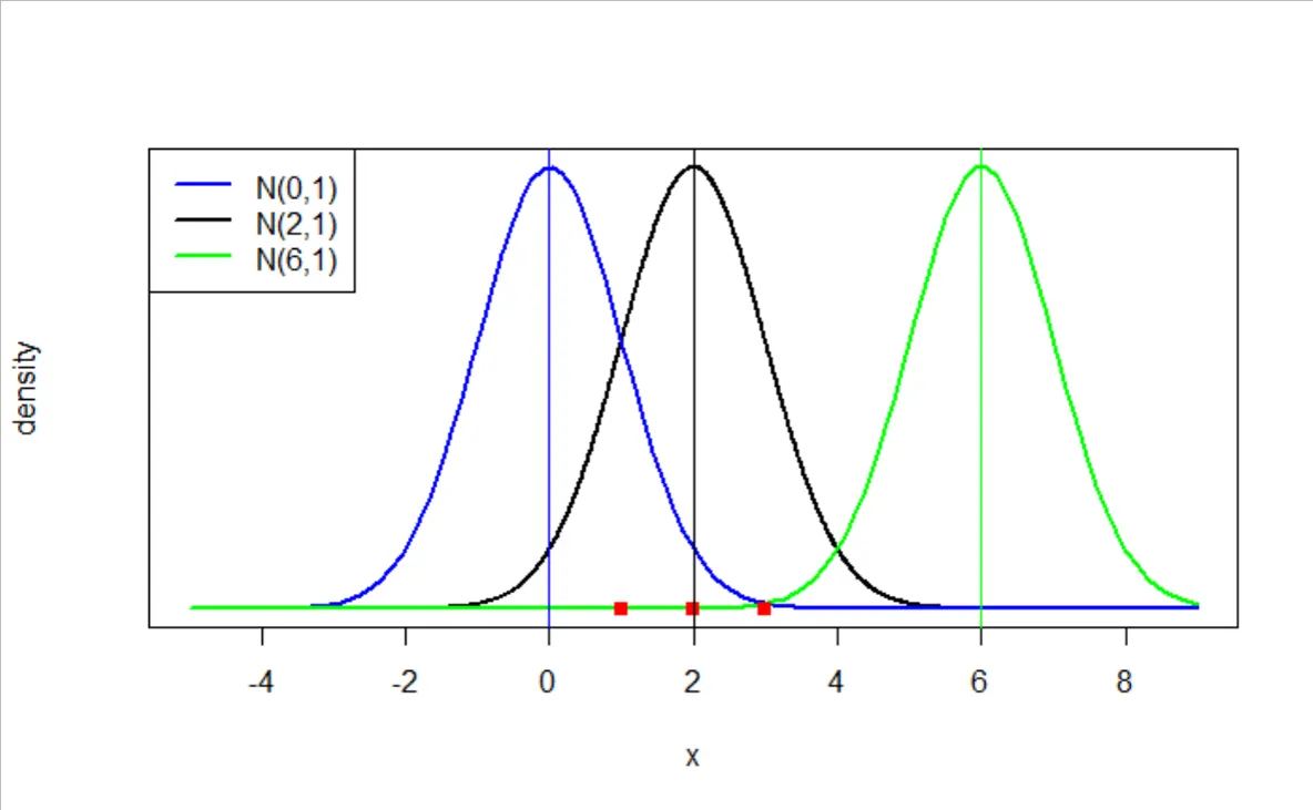
Training by MLE requires computing log P(x), which means evaluating that integral over z. For any z of reasonable dimension, integral has no closed form and exponentially expensive to approximate numerically.

The posterior P(z|x), which latent codes are consistent with a given observation x has the same problem. By Bayes' rule:

P(z|x) = P(x|z) P(z) / P(x)

The denominator is the same intractable integral. Evaluating the posterior requires P(x) and computing P(x) requires integrating over all z. There is no way out analytically.

Without the posterior, training is impossible: it is what tells the model which z values explain a given x.

Three Gaussian distributions with sample points

Source: towardsdatascience.com

Variational Inference

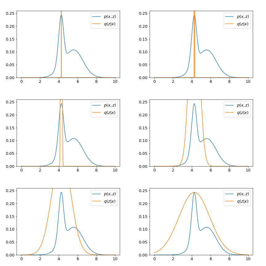
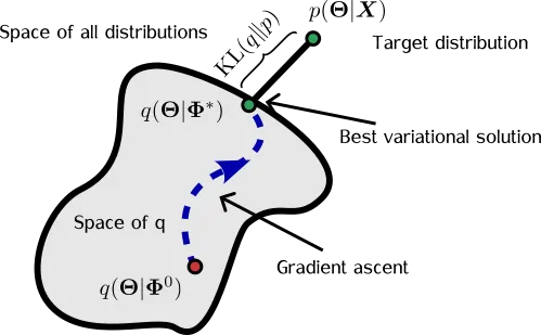
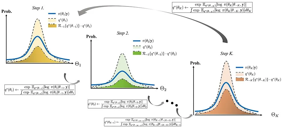
Rather than computing P(z|x) exactly, variational inference approximates it with a tractable distribution Q_φ(z|x), parameterized by φ. The goal is to find φ such that Q_φ(z|x) is as close as possible to P(z|x), where close is measured by KL(Q_φ ‖ P(z|x)).

Variational inference solution space diagram

Source: towardsdatascience.com

Minimizing KL(Q_φ ‖ P(z|x)) directly still requires evaluating P(z|x), so the problem is not solved yet. The key move is to rewrite the objective entirely in terms of quantities that are tractable.

Coordinate ascent variational inference steps

Source: en.wikipedia.org

The ELBO

Log P(x) decomposes exactly as:

log P(x) = ELBO + KL(Q_φ(z|x) ‖ P(z|x))

Since KL ≥ 0, the ELBO is always a lower bound on log P(x). Maximizing the ELBO over φ and θ does two things simultaneously: it pushes log P(x) up and it pulls Q_φ closer to the true posterior P(z|x), tightening the bound from below.

The ELBO expands into two interpretable terms:

ELBO = E_Q[log P(x|z)] — KL(Q_φ(z|x) ‖ P(z))

First term is reconstruction quality: how well does the model recover x from latent codes sampled under Q_φ? Second is a regularization penalty: how far is the approximate posterior from the prior P(z)?

Neither term requires evaluating P(z|x) or P(x). The intractable posterior disappears from the objective entirely.

Evidence, ELBO, and KL relationship

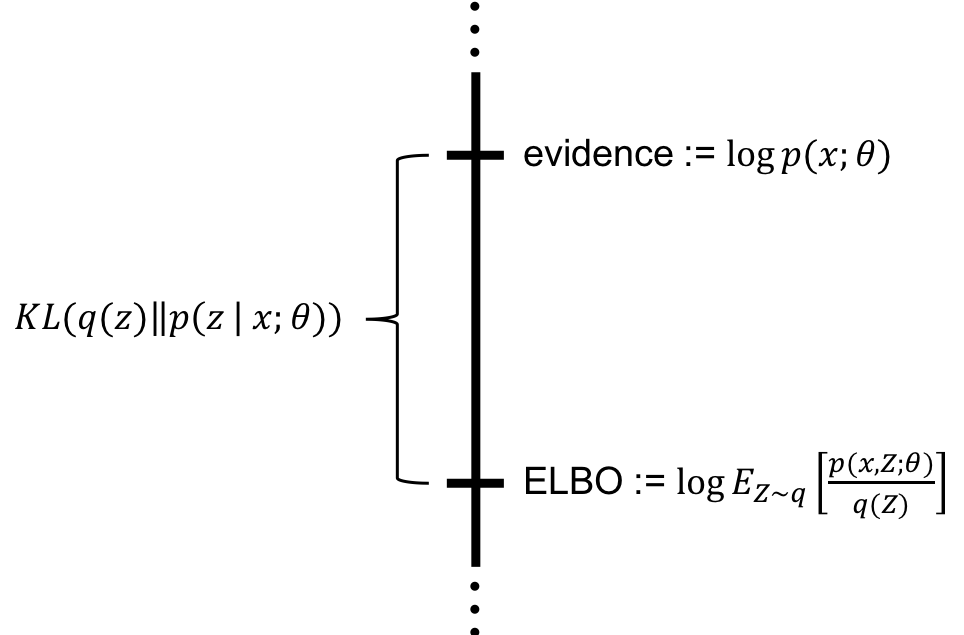
Source: mbernste.github.io

Training with the ELBO

Both φ and θ are optimized jointly by maximizing the ELBO. The generative model gets better at reconstructing x from z; the approximate posterior gets better at identifying which z values explain a given x.

Post 3 builds the concrete architecture on top of this: encoder network that outputs Q_φ(z|x), decoder network that outputs P(x|z) and reparameterization trick that makes backpropagation through the sampling step work.

A Note on Scope

This post is written for conceptual understanding, not mathematical rigor. Derivations, proofs and edge cases are intentionally omitted. The goal is to build enough intuition to follow the architecture decisions in the posts that follow. The references below cover the formal treatment for anyone who wants to go deeper.

References

- Langseth, H. & Nielsen, T. D. (2021). Probabilistic AI: Lecture 1 — Introduction to Variational Inference and the ELBO. SINTEF / Aalborg University.
- Jiang, Y. (2021). ELBO — What & Why. Yunfan's Blog.
- Adams, R. (2020). The ELBO without Jensen, Kullback, or Leibler. Laboratory for Intelligent Probabilistic Systems, Princeton University.
- Blei, D. M. (2011). Variational Inference [Lecture notes, COS 597C]. Princeton University.
- Ganguly, A. & Earp, S. W. F. (2021). An Introduction to Variational Inference. arXiv:2108.13083.
- Rainforth, T. (2022). Chapter 9, Part 2: Variational Inference [Lecture notes, Advanced Topics in Statistical Machine Learning, Hilary 2022]. University of Oxford.
- Rafailov, R. (2021). Variational Inference Tutorial. Stanford CS330.